Type a new column heading in a blank column to indicate the frequency limits that you want. For example, if you want to show a frequency distribution for every 10 units you would need to define that for Excel. The Frequency function refers to this limit as the 'Bin Array.' In the first cell under the column heading, type the number zero.

Creating a Histogram using FREQUENCY Function. If you want to create a histogram that is dynamic (i.e., updates when you change the data), you need to resort to formulas. In this section, you’ll learn how to use the FREQUENCY function to create a dynamic histogram in Excel.

In the next cell below that, enter the formula: '=B2+10' where 'B2' is the cell where you entered zero and '10' is the number of units you want to show for each section of your frequency distribution. After you type in the formula, but before you press 'Enter' the cell will be highlighted with a bold outline. Hold your mouse pointer over the lower, right corner of the cell so that it turns into a black cross. Click and drag downward to copy the formula until the last number shows the maximum limit for your frequency distribution. For example, if you are using a percentage scale, you would want to end at '100.' When you're done, press 'Enter.' Enter a column heading for the next column over and label it as 'Frequency Distribution.'

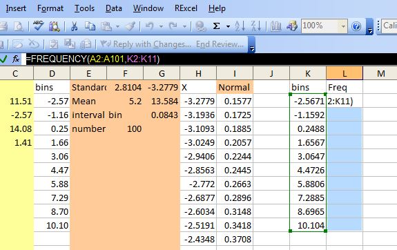
In the first blank cell under the heading, type the formula '=Frequency(' and then you will see in the formula bar the labels 'data_array' and 'bin_array.' Click 'data_array' and then click and drag on the spreadsheet to select all of the data cells. In this example it would be the cells in column 'A.' Type a comma which will highlight 'bin_array' in the formula bar. What replaced access for mac. Click and drag to highlight all of the values in for the frequency, in this example they would be in column 'B.' Press 'Enter.'

Scroll Bars in Excel I have used Excel for mac 2011 to demonstrate a spreadsheet from my Manpower Planning friend Tony that finds appraisal results and values. Excel 2010 copes equally well with what you are about to read about but the scroll bars look nicer on the mac!

One of the features Tony wanted me to include was what he called sliders: Excel users call them scroll bars or scrollbars. What follows is just PART of the work sheet I created: the work sheet starts here with some basic data on the employee being appraised. Says: Thanks for the question Rob.

Good news and bad news: all of these features from Excel are made to look drab! There is no way of making them more colourful except by means of VBA, I think. I don’t program with VBA so cannot really comment. The blue sliders you see are not really sliders: they are data bars created by using conditional formatting and you can choose any colour you like for that! I do have that file if you would like to see how to make the blue data bar.